Notes on Machine Learning with NN

A quick review of related concepts.

Table of Contents:

Basics
Classification
ML Applications
[ML Tools][#MLTools]
- [Tensorflow in a Nutshell: a Reading][#Tensorflow]
Summary

Basics

Questions: what is machine learning?

The fundamental goal of machine learning is to generalize beyond the examples in the training set.

(Machine learning is) the field of study that gives computers the ability to learn without being explicitly programmed – Arthur Samuel

A computer program is said to learn from experience E with respect to some class of tasks T and performance measure P, if its performance at tasks in T, as measured by P, improves with experience E. – Tom Mitchell

Key Elements of ML Algorithm

Representation: how to represent knowledge. Examples include decision trees, sets of rules, instances, graphical models, neural networks, support vector machines, model ensembles and others.
Evaluation: the way to evaluate candidate programs (hypotheses). Examples include accuracy, prediction and recall, squared error, likelihood, posterior probability, cost, margin, entropy k-L divergence and others.
Optimization: the way candidate programs are generated known as the search process. For example combinatorial optimization, convex optimization, constrained optimization.

Model Representation

A typical machine learning model:

Dataflow in a typical ML system

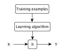
x^{(i)}	input variables, input features
y^{(i)}	output or target variable, to be predicted
(x^{(i)}, y^{(i)})	a training example
(x^{(i)}, y^{(i)}); (i = 1, …, m)	a training set
X	the input space
Y	the output space
h: X \rightarrow Y	a hypothesis function

Cost Function: how well does the hypothesis function fit the input data?

** Cost function ** measures the accuracy of the hypothesis function, e.g. mean square error function. Our objective is to get the lowest prediction error.

Parameter Learning via Gradient Descent

** Gradient descent ** estimates the parameters in the hypothesis function, by taking the (partial) derivatives of the the cost function. It repeatedly and simultaneously updates the parameters until convergence.

# compute gradients w.r.t. existing parameters
grad = function_SGD(x, w1, w2)

# compute new parameters
w1_ = w1 - step_size*grad
w2_ = w2 - step_size*grad

# update parameters
w1 = w1_
w2 = w2_

Difficulties:

step size, i.e. learning rate
gradient descent method, e.g. batch, online, stochastic

Classification

Goals

build a simple image classification pipeline, based on the k-Nearest Neighbor or the SVM/Softmax classifier.
understand the basic Image Classification pipeline and the data-driven approach (train/predict stages)
understand the train/val/test splits and the use of validation data for hyperparameter tuning.
develop proficiency in writing efficient vectorized code with numpy
implement and apply a k-Nearest Neighbor (kNN) classifier
implement and apply a Multiclass Support Vector Machine (SVM) classifier
implement and apply a Softmax classifier
implement and apply a Two layer neural network classifier
understand the differences and tradeoffs between these classifiers
get a basic understanding of performance improvements from using higher-level representations than raw pixels (e.g. color histograms, Histogram of Gradient (HOG) features)

Nearest Neighbor Classifier

Clustering is a type of unsupervised learning: input data samples have no output labels. For example, K-Nearest Neighbor (KNN)

K-NN’s success is greatly dependent on the representation it classifies data from, so one needs a good representation before k-NN can work well. They are very expensive to train, but once the training is finished it is very cheap to classify a new test example. This mode of operation is much more desirable in practice.

1 Nearest Neighbor classifier

import numpy as np
# input
Xtr, Ytr, Xte, Yte = loadData('path') # magic function
# training
nn = NearestNeighbor() # create a Nearest Neighbor classifier class
nn.train(Xtr, Ytr) # train the classifier on the training data and labels
# testing
Yte_predict = nn.predict(Xte) # predict labels on the test data
# print the classification accuracy: average number of examples that are correctly predicted, label matches
print 'accuracy: %f' % (np.mean(Yte_predict == Yte))
# the classifier
class NearestNeighbor(object):
  def __init__(self):
    pass

  def train(self, X, y):
    """ X is N x D where each row is an example. Y is N x 1 """
    # the nearest neighbor classifier simply remembers ALL the training data
    slef.Xtr = X
    self.ytr = y

  def predict(self, X):
    """ X is N x D where each row is an example, which we wish to predict label for """
    num_test = X.shape[0]
    # make sure the output type matches the input type
    Ypred = np.zeros(num_test, dtype = self.ytr.dtype)

    # loop over all test rows
    for i in xrange(num_test):
      # find the nearest training image to the i'th test image
      # using the L1 distance (sum of absolute value differences)
      distances = np.sum(np.abs(self.Xtr - X[i,:]), axis = 1)
      ## or using the L2 distance
      # distance = np.sqrt(np.sum(np.square(self.Xtr - X[i,:]), axis = 1))
      min_index = np.argmin(distances) # get the index with the smallest distance
      Ypred[i] = self.ytr[min_index] # predict the label of the nearest example
    return Ypred

K Nearest Neighbor classifier

Xval = Xtr[:1000, :] # take the first 1000 for validation
Yval = Ytr[:1000]
Xtr = Xtr[1000:, :] # keep last 49,000 for train
Ytr = Ytr[1000:]

# find Hyperparameters that work best on the validation set
validation_accuracies = []
for k in [1, 3, 5, 10, 20, 50, 100]:
  # use a particular value of k and evaluate on validation data
  nn = NearestNeighbor()
  nn.train(Xtr, Ytr)
  # assume a modified NearestNeighbor class that can take k as input
  Yval_predict = nn.predict(Xval, k = k)
  acc = np.mean(Yval_predict == Yval)
  print 'accuracy: %f' % (acc,)

  # keep track of what works on the validation set
  validation_accuracies.append((k, acc))

Disadvantages of k-Nearest Neighbor

Linear Classifier

Three core components of the (image) classification task: Score Function maps the raw image pixels to class scores (e.g. a linear function) Loss function measures the quality of a certain set of parameters (e.g. softmax vs SVM) Optimization finds the set of parameters W that minimize the loss function

3 key components in (image) classification task:

1. A (parameterized) score function maps the raw image pixels to class scores (e.g., a linear function $f(x_i,W) = Wx_i$)
1. A loss function L measures the quality of a particular set of parameters using certain scores (e.g., Softmax/SVM)
1. An optimization function finds the set of parameters W that minimize the loss function

Score Function

\[f(x_i, W, b) = W*x_i + b\]

binary Softmax classifier (also known as logistic regression)

Loss Function

loss function measures our unhappiness with outcomes, sometimes also referred to as the cost function or the objective function.

Multiclass SVM

\[L = \frac{1}{N} \sum_i \sum_{j\neq y_i} \left[ \max(0, f(x_i; W)_j - f(x_i; W)_{y_i} + \Delta) \right] + \lambda \sum_k\sum_l W_{k,l}^2\]

Code for the loss function, without regularization, in python, both unvectorized and half-vectorized form:

def L_i(x, y, W:
  """
  unvectorized version.
  - x
  - y
  - W
  """
  delta =
  score =

def L_i_vectorized(x, y, W):
  """
  half-vectorized implementation, where for a single example the implementation contains no for loops, but there is still one loop over the examples outside this function
  """
  delta =
  scores =
  margins =
  margins[y] =
  loss_i =
  return loss_i

def L(X, y, W):
  """
  fully-vectroized implementation:
  - X
  - y
  - W
  """
  delta =
  score =

Softmax

Compare

$ \sum_{\forall i}{x_i^{2}} $

$P(y = 1 \mid x; w,b) = \sigma(w^Tx + b)$, where $\sigma(z) = 1/(1+e^{-z})$

training dataset $x_i$, y_{i})\), where $ i = 1 \cdots N $

N examples each with dimensionality D K distinct categories

\[f(x,y) = x y\] \[f(x_i, W) = W*x_i\] \[\frac{\partial f(x,y)}{\partial x} = \frac{f(x+h,y) - f(x,y)}{h}\]

weights, parameters

Data preprocessing: mean subtraction, scale, [-1, 1]

Validation sets for Hyperparameter tuning

Optimization

Strategy 1: Random search: try out many different random weights and keep track of what works best.

# X_train is the data where each column is an example (e.g. 3073 x 50,000)
# Y_train are the labels (e.g. 1 x 50,000)
# L evaluates the loss function

bestloss = float("inf") # Python assigns the highest possible float value
for num in xrange(1000):
  W = np.random.randn(10, 3073) * 0.0001 # generate random parameters
  loss = L(X_train, Y_train, W) # get the loss over the entir training set
  if loss < bestloss: #track the best solution
    bestloss = loss
    bestW = W
  print 'In attemp %d the loss was %f, best %f' % (num, loss, bestloss)

# Assume X_test is [3073 x 10000], Y_test is [10000 x 1]
scores = Wbest.dot(Xte_cols) # 10 x 10000, the class scores for all test examples
# find the index with max score in each column, i.e. the predicted class
Yte_predict = np.argmax(scores, axis = 0)
# calculate accuracy (fraction of predictions that are correct)
np.mean(Yte_predict == Yte)
# returns 0.1555

Strategy 2: Random local search: tries to extend one foot in a random direction and take a step only if it leads downhill.

Start out with a random W
generate random perturbation $\deltaW$, if the loss at the perturbed $W + \deltaW$ is lower, then updata

W = np.random.randn(10, 3073) * 0.001 # generate random starting W
bestloss = float("inf")
for i in xrange(1000):
  step_size = 0.0001
  Wtry = W + np.random.randn(10, 3073) * step_size
  loss = L(Xtr_cols, Ytr, Wtry)
  if loss < bestloss:
    W = Wtry
    bestloss = loss
  print 'iter %d loss is %f' % (i, bestloss)
# returns 0.214

Strategy 3: Following the gradient: computes the best direction along which we should change our weight vector that is mathematically guaranteed to be the direction of the steepest descent. This direction will be related to the gradient of the loss function.

What is the gradient?

1-D functions, derivatives, the gradient is the vector of slopes for each dimension
x-D functions, partial derivatives, the gradient is the vector of partial derivatives in each dimension

How to compute the gradient?

numerical gradient: compute numerically with finite differences

def eval_numerical_gradient(f, x):
  """
  a naive implementation of numerical gradient of f at x
  - f is a function that takes a single argument
  - x is the point (numpy array) to evaluate the gradient at
  """
  fx = f(x) # evaluate function value at original point
  grad = np.zeros(x.shape)
  h = 0.00001

  # iterate over all indexes in x
  it = np.nditer(x, flags=['multi_index'], op_flags=['readwrite'])
  while not it.finished:

    # evaluate function at x+h
    ix = it.multi_index
    old_value = x[ix]
    x[ix] = old_value + h # increment by h
    fxh = f(x) # evaluate f(x+h)
    x[ix] = old_value # restore to previous value (!!!important)

    # compute the partial derivative
    grad[ix] = (fxh -fx) /h # the slope
    it.iternext() # step to next dimension

return grad

Compute gradient for the CIFAR-10 loss function at some random point in the weight space:

# a function that takes a single argument, the weights,
def CIFAR10_loss-fun(W):
  return L(X_train, Y_train, W)

 W = np.random.rand(10, 3073) * 0.001 # random weight vector
 df = eval_numerical_gradient(CIFAR10_loss_fun, W) # get the gradient

# the gradient tells the slope of the loss function along every dimension, we use it to make an update
loss_original = CIFAR10_Loss_fun(W) # original loss
print 'original loss: %f' % (loss_original, )

# effect of multiple step sizes
for step_size_log in [-10:1:-1]
  step_size = 10**step_size_log
  W_new = W - step_size*df
  loss_new = CIFAR10_loss_fun(W_new)
  print 'for step size %f new loss: %f' % (step_size, loss_new)

analytic gradient: compute analytically with Calculus

gradient descent mini-batch GD, stochastic GD (i.e. on-line gradient descent)

Linear Regression with One/Multiple Variables

Linear regression predicts a real-valued output based on an input value.

cost function

gradient descent for learning.

\[\begin{align} X &= [1, X_1 X_2 \cdots X_n] &= \begin{bmatrix} 1 &x_1^{(1)} &\cdots & x_n^{(1)} \\ 1 &x_1^{(2)} &\cdots &x_n^{(2)} \\ \vdots &\vdots &\ddots &\vdots \\ 1 &x_1^{(m)} &\cdots &x_n^{(m)} \end{bmatrix} \\ \theta &=\begin{bmatrix} \theta_0 \\ \theta_1 \\ \vdots \\ \theta_n \\ \end{bmatrix} \end{align}\]

i.e., $X_0 = 1$

Logistic Regression

Non-linear Classification with Neural Networks

Goals

write backpropagation code, and train Neural Networks and Convolutional Neural Networks.
understand Neural Networks and how they are arranged in layered architectures
understand and be able to implement (vectorized) backpropagation
implement various update rules used to optimize Neural Networks
implement batch normalization for training deep networks
implement dropout to regularize networks
effectively cross-validate and find the best hyperparameters for Neural Network architecture

Questions

what a neural network is really doing, behavior of deep neural networks
how it is doing so, when succeeds; and what went wrong when fails.
- explore low-dimensional deep neural networks when classifying certain datasets
- visualise the behavior, complexity, and topology of such networks
On an example dataset, with each layer, the network transforms the data, creating a new representation

Architecture

Biological motivation

# sigmoid activation function
def sigmoid(x):
  return 1.0/(1.0 + math.exp(-x))

class Neuron(object):
  # example of forward propagating a single neuron
  def forward(inputs):
    """ assume inputs and weights are 1-D numpy arrays and bia is a number """
    cell_body_sum = np.sum(inputs * self.weights) + self.bias
    firing_rate = sigmoid(cell_synapse)
    return firing_rate

Data and Loss Function

Learning and Evaluation

Case Study

Problem setting 1: linear dataset

1x + 2y + 3 z = 12

2x + 3y + 4z = 11

3x + 4y + 5z = 10

Formulate with numpy

import numpy as np

A*X = b
A = np.array(np.mat(‘1 2 3; 2 3 4; 3 4 5’))
A = np.array([[1, 2, 3], [2, 3, 4], [3, 4, 5]])
X = np.transpose(np.array([x, y, z]))
# visualize the data
TBD

Problem setting 2: non-linear (spiral) dataset

import numpy as np

N = 100 # number of points per class/spiral wing
D = 2  # dimensionality
K = 5  # number of spiral wings
X = np.zeros((N*K)) # data matrix (each row is a single training example)
y = np.zeros(N*K, dtype='uint8') # class labels
for j in xrange(K):
  ix = range(N*j, N*(j+1))
  r = np.linspace(0.0, 1, N) # radius
  t = np.linspace(j*4, (j+1)*4, N) + np.random.randn(N)*0.2 # theta
  X[ix] = np.c_[r*np.sin(t), r*np.cos(t)]
  y[ix] = j
# visualize the data
plt.scatter(X[:,0],X[:,1], c=y, s=40, cmap=plt.cm.Spectral)

Loss function

def L_ivectorized(x, y, w):
    scores = w.dot(x)
    margins = np.maximum(0, scores - scores[y] +1)
    margins[y] = 0
    loss_i = np.sum(margins)
    return loss_i

“Sigmoid Function,” also called the “Logistic Function”:

Convolutional Neural Networks

Recurrent Neural Networks

Goals

Implement recurrent networks, and apply them to image captioning on Microsoft COCO.
Understand the architecture of recurrent neural networks (RNNs) and how they operate on sequences by sharing weights over time
Understand the difference between vanilla RNNs and Long-Short Term Memory (LSTM) RNNs
Understand how to sample from an RNN at test-time
Understand how to combine convolutional neural nets and recurrent nets to implement an image captioning system
Understand how a trained convolutional network can be used to compute gradients with respect to the input image
Implement and different applications of image gradients, including saliency maps, fooling images, class visualizations, feature inversion, and DeepDream.

Continuous Visualization of Layers

A linear transformation by the “weight” matrix
A translation by the vector
Point-wise application of e.g., tanh.

ML Applications

Toy Example

Audio: Human Speech and Language Processing

polyphonic sound event detection in real life recordings

Motivation It is a way of x, which is critical for x, and x.

Problem statement The core problem studies is:

Given x, where x, and we want to compute/debug x.

Expressions and interpretation of the problem

Vision: Image and Video Processing

Tools for ML

“If a human expert couldn’t use the data to solve the problem manually, a computer probably won’t be able to either. Instead, focus on problems where a human could solve the problem, but where it would be great if a computer could solve it much more quickly.”

Tensorflow in a Nutshell: a Reading

Summary

Historical Context

cat & edges, how brain neurons work, 1981, 1963
1966 A.I. Computer Vision

Some Basic Concepts

ML by Tasks

Supervised learning
- Nearest neighbor
- Linear classifiers
  - Linear regression with one/multiple variable
  - Logistic Regression
  - Support vector machines
  - Naive Bayes classifer
- Support vector machines
- Decision trees
  - C4.5
  - Random forests
  - CART
- Hidden Markov models
- Artificial neural network
  - Hopfield networks
  - Boltzmann machines
  - Restricted Boltzmann machines
- Random Forest
- Conditional Random Field
- ANOVA
- BayEsian network
- …
Unsupervised learning
- Artificial neural network
  - self-organizing map
- Clustering
  - K-means clustering
  - Fuzzy clustering
- …
Deep learning
- deep belief networks
- deep Boltzmann machines
- deep Convolutional neural networks
- deep Recurrent neural networks
Semi-supervised learning (…)
Reinforcement learning (…)

Organization may vary across subjects, this list is mainly from Coursera (ML basics) and wiki (ML concepts)

ML by Outputs

Classification
Regression
Probability Estimation
Clustering
Dimensionality Reduction